An implementation of the Paper "High Performance By Example Noise"

Notes:

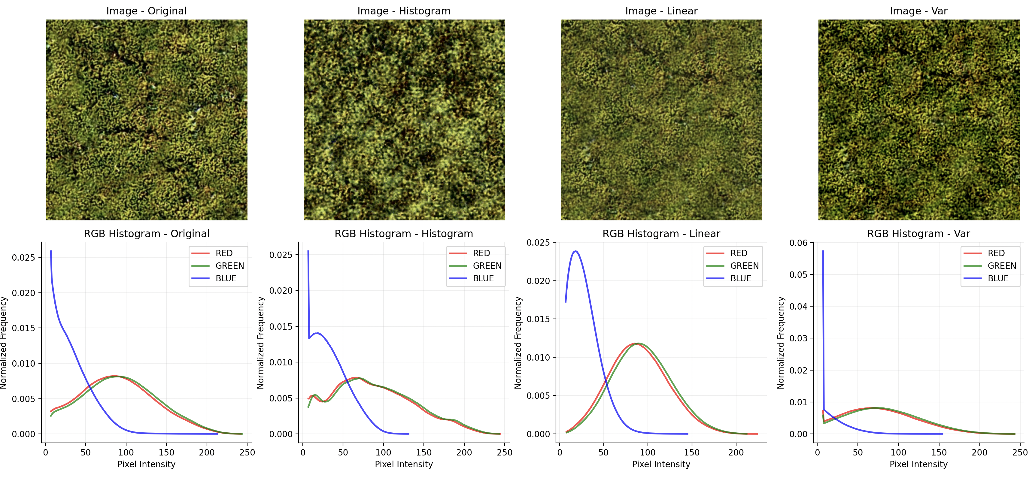
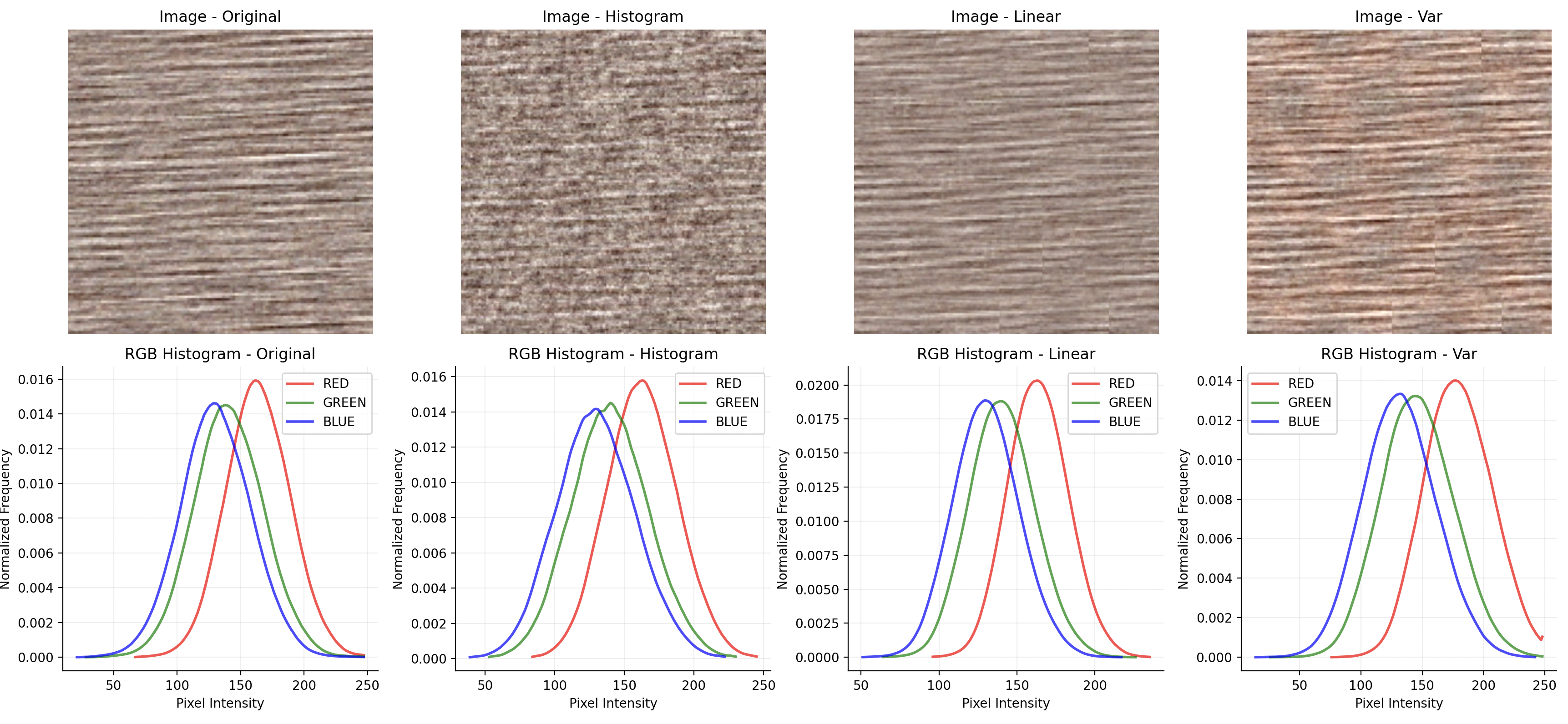
• A quick sketch of the paper is: input (low-res texture) -gaussianize-> gaussian_image -blending-> blended gaussian - inverse_gaussianize-> high-res texture. So ideally you can get an infinite resolution texture with similar histogram as the input.

• The implementation is now an offline compute + real-time LUT approximate solution. It uses PyOT to gaussianize the input texture (which should be a exact solution), OpenGL (GLSL) to perform the blend. And you can either use OT (written in python script to perform the inverse transformation) or OpenGL (approximated OT) to perform the inverse transformation.

  • The inverse transformation is approximated by Inverse Histogram Equalization per channel. However, the input has to be under decorrelated color space. Otherwise it wouldn’t account for color correlations properly. Thus, a PCA-like process is used to decorrelate the color space. (This is referenced from author’s implementation. https://eheitzresearch.wordpress.com/738-2/)

• If you’re only interested in the shader blending process, check this out:

  • https://www.shadertoy.com/view/MdyfDV

To use the program:

• The dependencies of python environment is under ./requirements.txt

  • To use (Python version 3.9.6)

  • pip install -r requirements.txt

• The dependencies of OpenGL environments are listed in CMakeLists.txt

• Run gaussianize.py to get the gaussianized image of the input. The output will be under /gaussian_output/ by default, with _g naming suffix.

  • The gaussianization step uses PyOT library for a batched Optimal Transport calculation. Usually it will take more than 32 Gigs of RAM if we are going to do a gaussianization on a 256 x 256 RGB image.
  • The batched solver finishes this step in 10 seconds with a 10-core CPU.

• Insrc/NoiseSynth.hpp, change the noiseTexturePath,gaussianTexturePath to be the original noise texture path, and the gaussianized noise texture path.

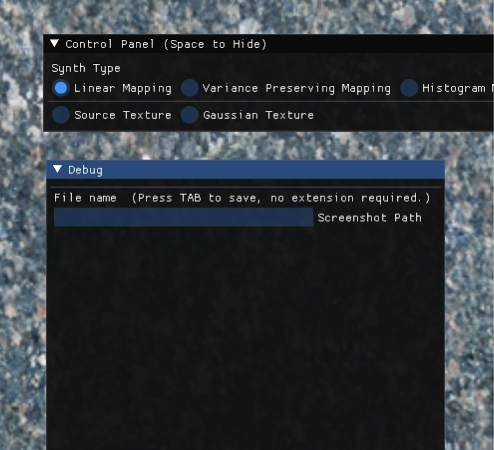
• You can either feed the blended gaussian result (from screenshot function) to the inverse_gaussianize.py file to get the final result (256 x 256 to 1024 x 1024 takes 2 min for inverse optimal transport), or tick “Histogram Mapping” in the GUI to see an approximated result (real-time).

• Choose from different blending method.

  • Press space to hide GUI
  • Press tab to take a screenshot (as the input for inverse transform), the screenshot will be saved to your input path (by default it will be under /result folder)
  

Bugs / Artifacts of Implementation

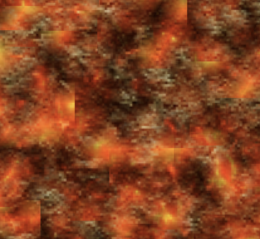
• The blending might gets horizontal or vertical artifacts for some texture (i.e. not seamless).

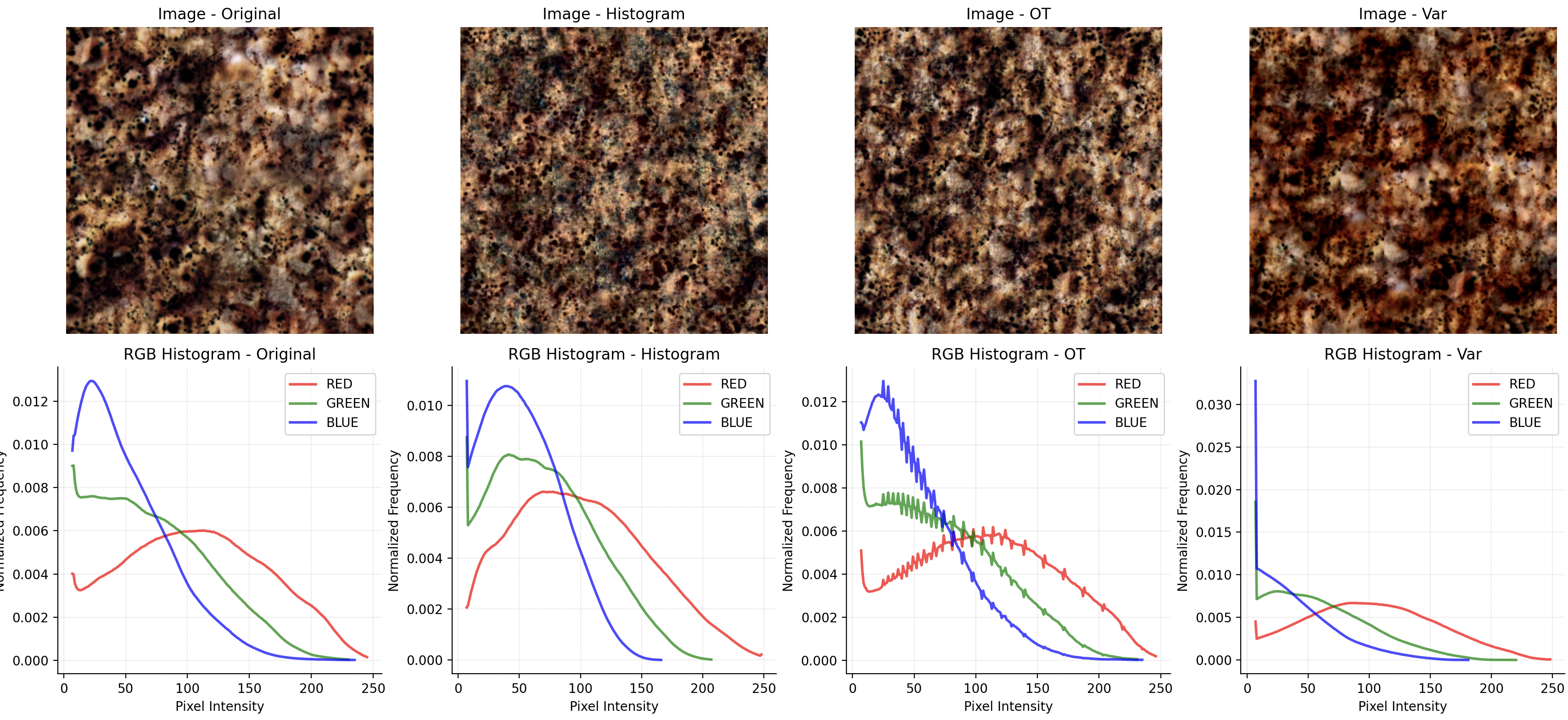
• The Optimal Transport method in my implementation makes the final histogram look squiggly (see results below).

Files:

• image_scaler

  • Simple image scale function

• image_visualizer

  • Image visualization functions including histograms and difference between images

• lut_visualizer

  • A tool to visualize LUT

• gaussianize

  • Gaussianize the input image using optimal transport. (See 4.1 / 4.2 of the paper)
    • Use a batched implementation to avoid OOM.

• inverse_gaussianize

  • Inverse transform the gaussianized image to input-like texture.
    • Current implementation uses optimal transport

• /src/shader/synth.fs

  • Simplex interpolation and LUT lookup

• /src/Precompute.hpp

  • Computation functions for inverse transformation and color space decorrelation.
    • Ref: https://eheitzresearch.wordpress.com/738-2/

• /src/Setup.hpp

  • Doing pre-computations and texture handling, initialization.

• /src/NoiseSynth.cpp

  • Main rendering loop and event handling.

Results:

Bad Examples:

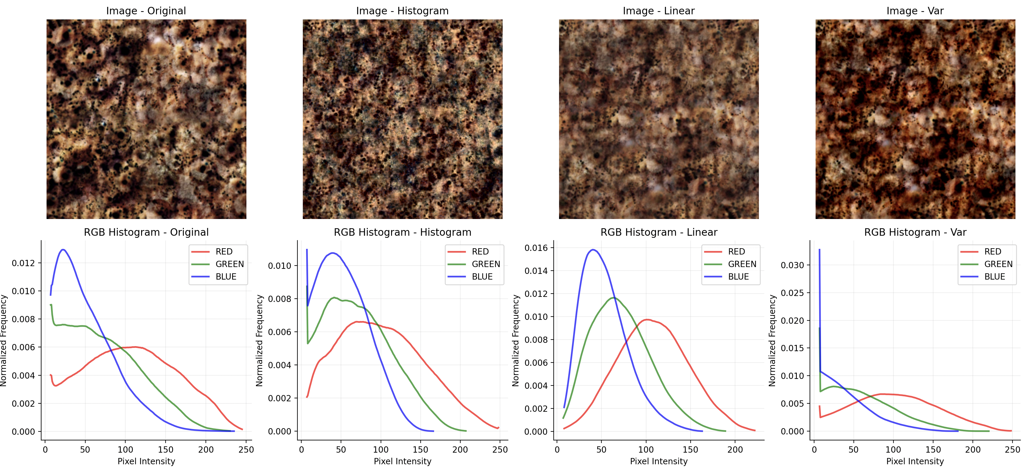
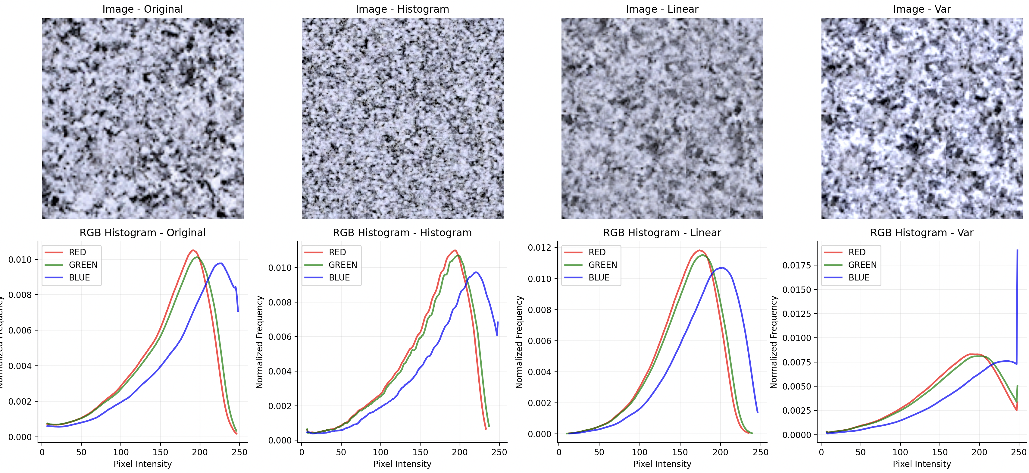
In the discussion section, the author mentioned that it fails if the input has a very strong pattern.

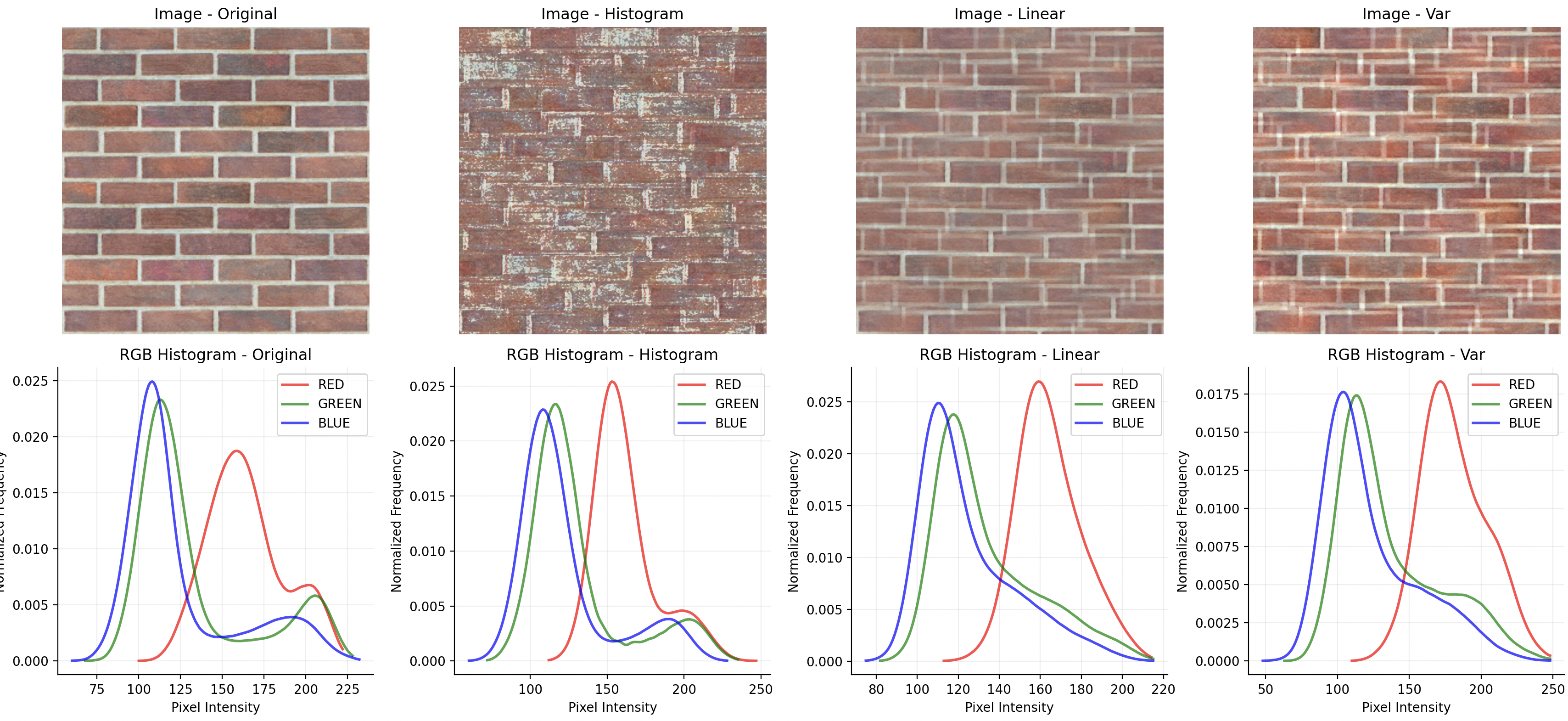
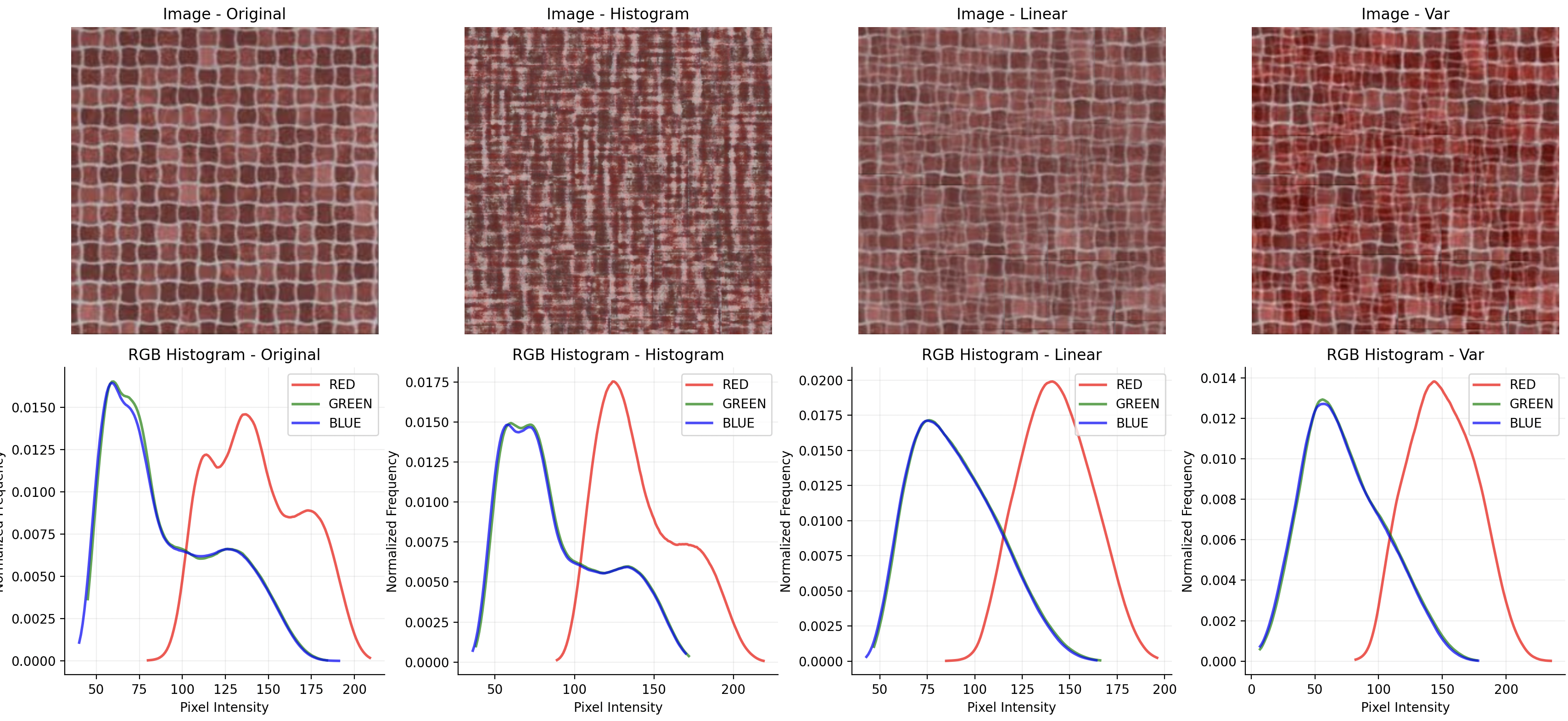
Also, since the inverse transformation is approximated without performing OT, there can be some difference between OT and the histogram-preserving blend.